Gurita: a command line data analytics and plotting tool

Gurita is a command line tool for transforming, analysing, and visualising tabular data in CSV or TSV format.

At its core Gurita provides a suite of commands, each of which carries out a common data analytics or plotting task. Additionally, Gurita allows commands to be chained together into flexible analysis pipelines.

It is designed to be fast and convenient, and is particularly suited to data exploration tasks. Input files with large numbers of rows (> millions) are readily supported.

Gurita commands are highly customisable, however sensible defaults are applied. Therefore simple tasks are easy to express and complex tasks are possible.

Gurita is implemented in Python and makes extensive use of the Pandas, Seaborn, and Scikit-learn libraries for data processing and plot generation.

Simple example

The following examples use the iris.csv dataset as input. The file contains 150 data rows (plus one heading row) and 5 columns. A pretty display of the first and last 5 rows of the data can be viewed using the following command:

cat iris.csv | gurita pretty

The command generates the following output that is displayed on the terminal:

 sepal_length  sepal_width  petal_length  petal_width   species
          5.1          3.5           1.4          0.2    setosa
          4.9          3.0           1.4          0.2    setosa
          4.7          3.2           1.3          0.2    setosa
          4.6          3.1           1.5          0.2    setosa
          5.0          3.6           1.4          0.2    setosa
          ...          ...           ...          ...       ...
          6.7          3.0           5.2          2.3 virginica
          6.3          2.5           5.0          1.9 virginica
          6.5          3.0           5.2          2.0 virginica
          6.2          3.4           5.4          2.3 virginica
          5.9          3.0           5.1          1.8 virginica

[150 rows x 5 columns]

The following command generates a box plot from iris.csv, such that the Y-axis represents the sepal_length numerical column, and the X-axis is grouped by the species categorical column. The goal of this plot is to show the distribution of sepal length of the three different species of iris flowers contained in the data set.

cat iris.csv | gurita box -x species -y sepal_length

The above command generates an output file called box.species.sepal_length.png containing the following figure:

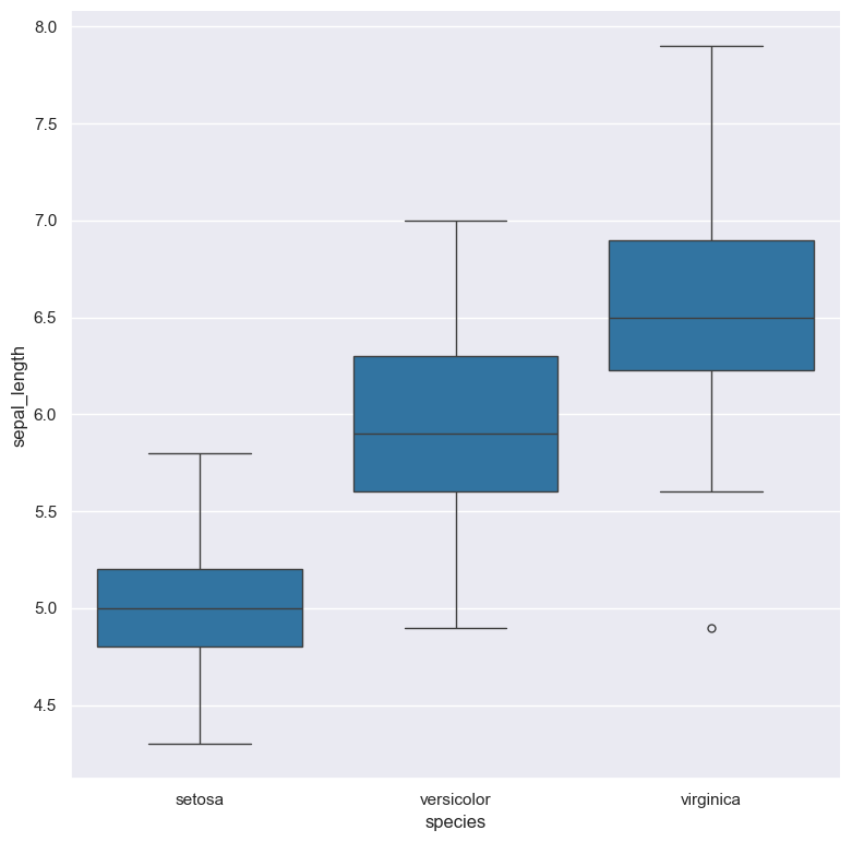
If we wanted to see the median value of sepal_length for each species we can do this with the following groupby command:

cat iris.csv | gurita groupby --key species --val sepal_length --fun median

species,sepal_length_median
setosa,5.0
versicolor,5.9
virginica,6.5

You can see that the corresponding median values match up with the values shown in the box plot.

Advanced example

The next example illustrates Gurita’s ability to chain commands together:

cat iris.csv | gurita filter 'species != "virginica"' \
                      + sample 0.9 \
                      + pca \
                      + scatter -x pc1 -y pc2 --hue species

The above command has been written on mulitple lines for clarity. Note that the backslash \ indicates a line break in the command line syntax.

Equivalently, the same command can be written in a single line, like so (where backslashes are no longer required):

cat iris.csv | gurita filter 'species != "virginica"' + sample 0.9 + pca + scatter -x pc1 -y pc2 --hue species

In the command line syntax supported by Gurita, the plus sign + separates each command in a chain. This notation is fairly novel to Gurita and not something commonly seen in other command line programs.

Input is read from the file called iris.csv on standard input and data is passed from left to right in the chain. Commands can modify the data as it is passed along.

In this example there are four commands that are executed in the following order:

1. The filter 'species != "virginica"' command selects all rows where species is not equal to virginica.

2. The filtered rows are then passed to the sample 0.9 command which randomly selects 90% of the remaining rows.

3. The sampled rows are then passed to the pca command which performs principal component analysis (PCA), yielding two extra columns in the data called pc1 and pc2.

4. Finally the pca-transformed data is passed to the scatter -x pc1 -y pc2 --hue species command which generates a scatter plot of pc1 and pc2 (the first two principal components), and colours the points in the plot based on the categorical species column.

The output of this entire Gurita command is the scatter plot below that is saved in a file called scatter.pc1.pc2.species.png

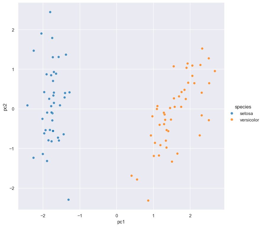
An interesting aspect of this example is that additional columns are added to the data in the pca step, and these extra columns are then used to define the axes of the following scatter plot.

Command chaining allows complex transformations to be combined together and makes Gurita a very powerful tool.