pca
Perform principal component analysis (PCA) on numerical columns in a dataset.
PCA is a popular dimensionality reduction technique. It transforms data into new coordinates such that most of the variation in the data is described with fewer dimensions than the original data.
The pca command adds new columns to the dataset representing the computed principal components.
PCA does not work with missing values, so rows with missing (NA) values in the analysed columns are automatically removed before PCA is applied.
Usage
gurita pca [-h] [-c NAME [NAME ...]] [--prefix PREFIX] [-n COMPONENTS]
Arguments
Argument |
Description |
Reference |
|---|---|---|
|
display help for this command |
|
|
apply PCA to these columns |
|
|
number of principal components to generate (default: 2) |
|
|
choose a column name prefix for new PCA columns (default: pc) |
Simple example
The following command computes the first two principal components of the numerical columns in the iris.csv file:
gurita pca < iris.csv
The output is quite long so we can adjust the command to look at only the first few rows using the head command:
gurita pca + head < iris.csv
The output of the above command is as follows:
sepal_length,sepal_width,petal_length,petal_width,species,pc1,pc2
5.1,3.5,1.4,0.2,setosa,-2.2645417283948928,0.5057039027737834
4.9,3.0,1.4,0.2,setosa,-2.0864255006161576,-0.6554047293691353
4.7,3.2,1.3,0.2,setosa,-2.367950449062523,-0.3184773108472487
4.6,3.1,1.5,0.2,setosa,-2.3041971611520085,-0.5753677125331953
5.0,3.6,1.4,0.2,setosa,-2.388777493505642,0.6747673967025161
Two new columns are added to the output dataset, called pc1 and pc2, representing the first and second principal components
of the numerical columns in the input data.
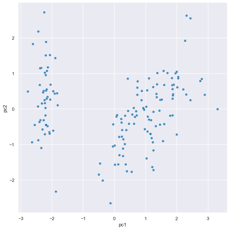
It is useful to visualise the principal components in a scatter plot, which can be achieved by chaining
with the scatter command:
gurita pca + scatter -x pc1 -y pc2 < iris.csv
The output of the above command is written to scatter.pc1.pc2.png:
Getting help
The full set of command line arguments for pca can be obtained with the -h or --help
arguments:
gurita pca -h
Perform PCA on specified columns
-c NAME [NAME ...], --col NAME [NAME ...]
By default, if no column names are specified, PCA is performed on all of the numerical columns in the dataset.
However it is possible to perform PCA on a specific subset of columns via the -c/--col argument.
For example, the following command performs PCA on just the columns sepal_length, sepal_width, and petal_length (and hence ignores the petal_width column):
gurita pca -c sepal_length sepal_width petal_length < iris.csv
Note
Non-numeric columns will be ignored by pca even if they are specified as arguments to -c/--col.
Choose the number of principal components to generate
-n COMPONENTS, --ncomps COMPONENTS
By default the pca command will computer the first two principal components on the input dataset.
This can be adjusted using the -n/--ncomps argument.
For example, the following command generates the first three principal components of all the numerical columns in the iris.csv file:
gurita pca -n 3 < iris.csv
The output is quite long so we can adjust the command to look at only the first few rows using the head command:
gurita pca -n 3 + head < iris.csv
The output of the above command is as follows:
sepal_length,sepal_width,petal_length,petal_width,species,pc1,pc2,pc3
5.1,3.5,1.4,0.2,setosa,-2.2645417283948928,0.5057039027737834,-0.12194334778175248
4.9,3.0,1.4,0.2,setosa,-2.0864255006161576,-0.6554047293691353,-0.2272508323992485
4.7,3.2,1.3,0.2,setosa,-2.367950449062523,-0.3184773108472487,0.05147962364496831
4.6,3.1,1.5,0.2,setosa,-2.3041971611520085,-0.5753677125331953,0.09886044443740284
5.0,3.6,1.4,0.2,setosa,-2.388777493505642,0.6747673967025161,0.021427848973115345
Note
Let N be the number of rows and C be the number of numerical columns considered in a PCA.
Let M = minimum(N, C).
The number of principal components must be <= M.
An error message will be generated if this condition is not met.
For example, there are 150 rows and 4 numerical columns in the iris.csv. Therefore
a PCA applied to all the numerical columns must not request more than 4
principal components, because 4 is the minimum(150, 4). Thus the following
command will generate an error:
gurita pca -n 5 < iris.csv
Choose a column name prefix for new PCA columns
--prefix PREFIX
The pca command adds extra numerical columns to the dataset to store the values for the computed principal components.
The principal components are integers from 1 upwards (1, 2, 3, …). The names of these extra columns are constructed by adding the preix pca
on to the number of the component, for example pc1 for the first component, pc2 for the second component and so on.
This can be changed with the --prefix argument.
The following command specifies that comp should be used as the prefix for the newly added columns:
gurita pca --prefix comp < iris.csv
By chaining this command with head we can inspect the first few rows of the output:
gurita pca --prefix comp + head < iris.csv
The output of the above command is as follows:
sepal_length,sepal_width,petal_length,petal_width,species,comp1,comp2
5.1,3.5,1.4,0.2,setosa,-2.2645417283948928,0.5057039027737834
4.9,3.0,1.4,0.2,setosa,-2.0864255006161576,-0.6554047293691353
4.7,3.2,1.3,0.2,setosa,-2.367950449062523,-0.3184773108472487
4.6,3.1,1.5,0.2,setosa,-2.3041971611520085,-0.5753677125331953
5.0,3.6,1.4,0.2,setosa,-2.388777493505642,0.6747673967025161
Observe that the two new principal component columns are called comp1 and comp2 respectively.